An explanation of aerodynamic lift

Esquema de tópicos/temas

• General

  Author: Peter Higgins, PhD                                                                                                   Updated August 2023

  Keywords: aerodynamics, lift, wake turbulence, Bernoulli, flow equations, openFOAM, XFoil, JavaFoil
  

  Intended for students 14+

  Prerequisites: some basic science, but there are few equations here, whats really needed is curiosity and an interest in airplanes.
  

  Lift is explained as resulting from circulation, and is not the consequence of the widely held but the erroneous equal transit time hypothesis. Both wind tunnel observations and the author's own wing modeling in OpenFoam are used to explain what really happens. It is seen that the vortices that are a danger to following aircraft taking off behind jumbo-jets are also explained as a necessary result of lift generation. This lecture puts the Bernoulli equation in lift generation in proper perspective. The presence of lift in other atmospheres, such as found on Mars, is discussed.
  

  This lesson is intended for high school and lower university levels. It introduces students to the excellent book on the subject by Clancy. Hopefully, some will be inspired to learn computer modeling by looking at the results presented.

  
  

  Aerodynamic lift refers to the force pushing upwards that is generated on an airplane wing when it moves through the atmosphere. In short, lift keeps the airplane flying, without lift planes can not fly even with powerful engines. Rockets can, but that is another story.

  Lift can be understood by wind tunnel observations. When a wing is angled into the flow slightly upward, the flow is always faster flow over the top than under it. According to the principle of conservation of energy, such faster flow lowers the top surface pressure forcing (or sucking) the wing up. This principle was discovered by Daniel Bernoulli and will be discussed later.

  A question remains, however, why is the top flow faster when lift occurs? A common reason presented for this phenomenon is that the path over the top surface is longer than the path along the bottom surface so that flow over the top speeds up to join its counterpart at the trailing edge. This is wrong because as observed in wind tunnels, when flow recombines the top flow does not meet its counterpart that split at the front. The real reason is described in this lesson.

  Anticipating that some students will want to learn more about the performance of wings, known as airfoils, this lesson identifies three programs available for free that can be run by high school students to quantify lift for different airfoils. Airfoil shapes for different airplanes, like the Boeing 747, can be downloaded from the Internet. Analyzing wing performance could be a great Senior project.

  Lastly, since this lecture has been done with space exploration in mind, the lift of NASA's Martian helicopter is studied. It is noteworthy that it actually flew successfully because the Martian atmosphere is so thin compared to the Earth's. You can run the programs discussed in this lesson to see for yourself.
  

  
  

• Introduction

  

  
  

  Let us begin:

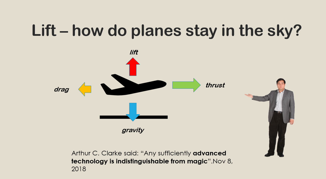
  We start by drawing a free-body diagram to visualize all the forces acting on an airplane. Lift forces hold the airplane up, while thrust from engines move it forward. Lift forces counteract the force of gravity. A 747 jumbo jet weighs up to 970,000 pounds at take off, so the forces of lift for it must be greater than that. But like gravity, the source of lift is mysterious. As Arthur Clarke said “Any sufficiently advanced technology is indistinguishable from magic”.   

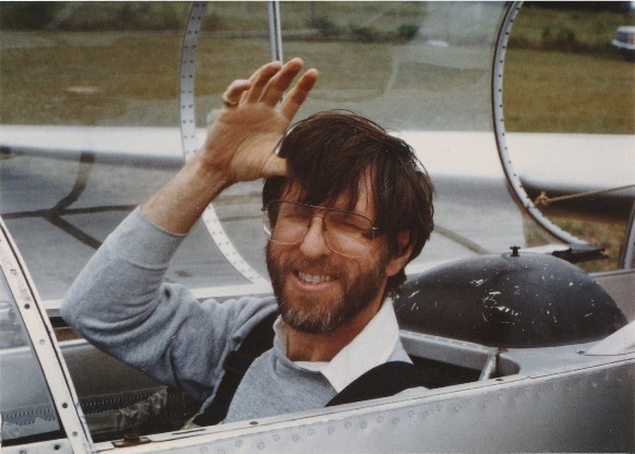
  I am Dr. Peter Higgins.  I used to fly sailplanes and have studied their wings with computer models. I have learned how lift forces develop. I’ve produced this lecture to explain what I have learned.

  
  

• How is lift studied
  There are two ways to study lift: the first is observation of flow around models in wind tunnels, the second is by simulation with computer programs.
  

  
  

  Wind tunnel testing

  
  

  
  

  
  

  
  

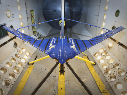  Wind tunnels can be very impressive facilities with huge tubes containing an instrumented  test chamber. Air is blown into the tubes by enormous fans then the tubes get smaller to further speed up the flow.. Baffles straighten the flow into parallel streams. The object being tested can be a wing or a model airplane as shown in this figure.
  

  
  

  Wind tunnel flow results

  
  

  Air flow captured by cameras through ports in the test chamber shows that for a slightly inclined wing (the inclination is called angle of attack) the flow splits into a portion which flows up over the top of the wing and into a portion which flows under the wing.  However, if the angle of attach is too great, the wing stalls and flow over the top separates from the wing and does not join with flow from the bottom. In this case lift is destroyed, gravity takes over, and the plane nosedives.

  When lift happens, two observations are always made: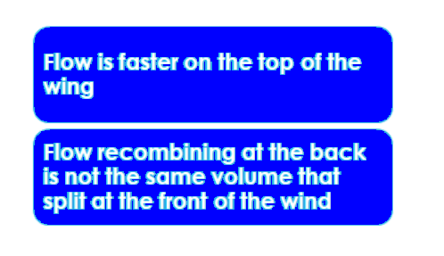
  

  
  

  
  

  1 Airflow is faster on the top of the wing than it is under the wing.

  2 The airflow from the top is not from the same air volume that split in the front.

  Observation 1 is important for  understanding lift because when flow is faster its pressure is lower. Observation 1 is the same as stating that the pressure on the top of the wing is lower than the pressure on the bottom. This pressure difference forces the wing upward opposing gravity. We would be done understanding lift if we understood why the top flow was faster.

  Observation 2 is critical in understanding lift. A popular, but incorrect theory claims that the faster flow on the top surface is the result of the top path being longer compared to the bottom path, and because the two paths are crossed by the split fluid parcels in equal time. This theory depends on the notion that the flow volumes that split at the front have to recombine with themselves as if this was the consequence of conservation of mass.  It isn't, and by placing dye markers in the upstream flow it's clear to any observer that this recombination constraint doesn't happen. This incorrect theory has a name: the equal transit time fallacy.

  Without the equal transit time theory, there is no apparent reason to explain the faster flow. There must be another mechanism to explain it.

  Returning to observation 1: the inverse relationship between flow speed and flow pressure is widely attributed to Daniel Bernoulli.

  
  

• Bernouilli's equation

  For any point in a flow:
  

  Pressure/density + gravitational constant · height + Velocity squared/2 = constant

  Each of these terms is an energy: the first is called flow energy, the second, potential energy, the third is kinetic energy. According to conservation of energy the sum these three terms at any point in the flow equals the sum of these terms at any other point. As a consequence, if the velocity increases from point 1 to point 2, the pressure must decrease at point 2. Daniel Bernoulli is credited with this discovery.

  
  

  Daniel Bernoulli came from a famous family of scientists; he was a mathematician and a Doctor. In his medical practice, he pioneered the measurement of blood pressure by inserting glass tubes in patient’s arms noting the height reached by the blood in the tube– if the patient’s blood was flowing normally, this height was low, but, if the height was high, the blood wasn’t flowing well.  But, Bernoulli never published the equation above that is attributed to him, it was his father’s student, the brilliant Leonhard Euler who did some years later. According to Euler,  along any streamline the sum of energies resulting from fluid pressure, height and velocity must be the same. When the fluid slows down at the same height, the pressure goes up, and vice-versa. It is now known that this relationship comes from conservation of energy. P/ρ is the flow energy, gz is potential energy and v²/2 is the flow's kinetic energy. By conservation of energy the sum of these values is the same anywhere in a non viscous flow. It is left to the student to show the units of each term equate to energy.
  

  
  

• Computer modeling of flow
  The video clip below is an animation from openFlow of a NACA airfoil in Earth's atmosphere for very small timesteps showing the development of low pressure (blue) along the top of the wing in just a fraction of a second (each timestep is a tenth of a second). The black lines are contours of pressure change. When the spacing between contours is small, the change is greater. (called a gradient) This animation shows that the low pressure that develops dominates, and lift occurs.
  

  
  

   

  
  

  
  

  
  

  
  

  Just four equations describe the variation of  pressure, density, temperature and velocity in a fluid flow such as in the track of hurricanes, or around wings in flight. The process of solving these equations in a flowing fluid is called numerical analysis, and is done in time steps. The results presented in the next slides come from OpenFoam. After several hours of computer time to simulate a few minutes of actual flow across the wing, results for the problem variables such as pressure and velocity can be visualized by graphics software.

  
  

  Click on the graphic above to see the development of lift as seen by low pressure (blue) being established on the top of the airfoil while high pressure occurs on the bottom. Once the equations are solved for an airfoil moving through the fluid (Earth's atmosphere) with enough angle of attack for lift, pictures of the final pressure and velocity can be examined. These are shown next:
  

  
  

  
  

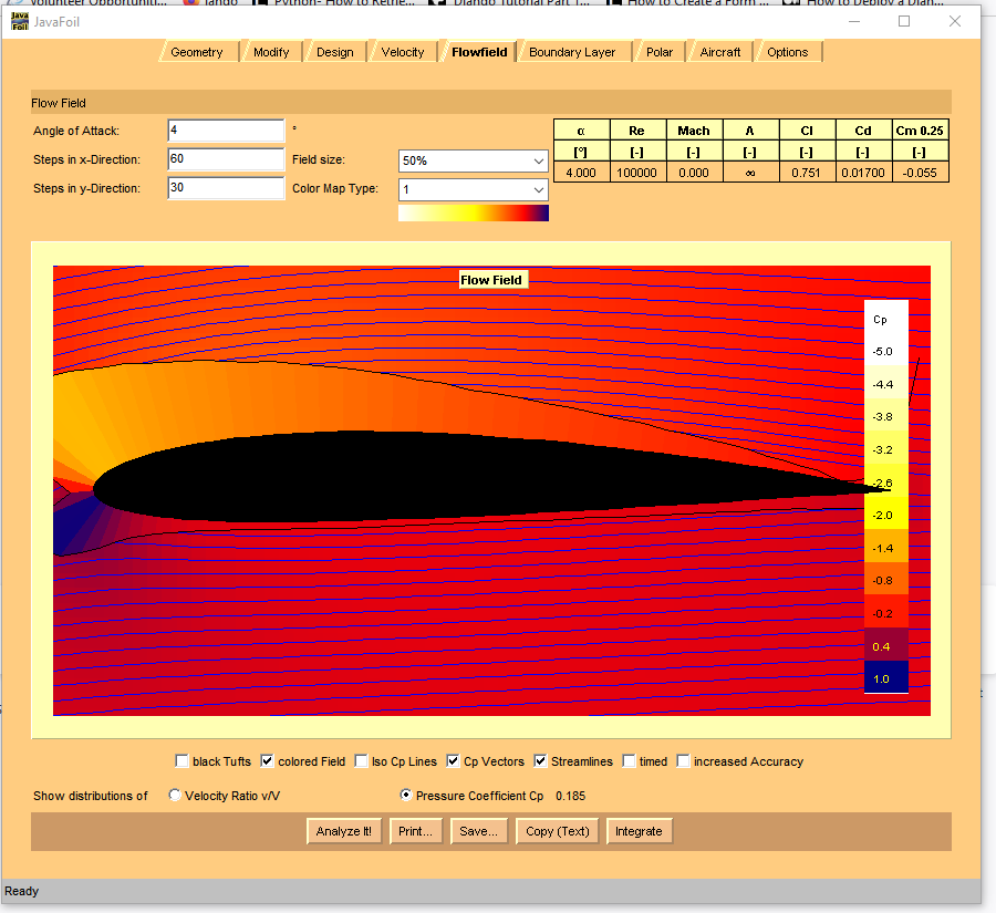
  Modeled pressure

  
  

  
  

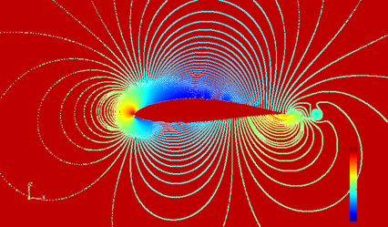  High pressure is red-yellow, low pressure appears blue.
  

  The modeled pressure in the flow around the airfoil section shows high pressure at the leading edge of the airfoil, and at the underside of the trailing edge. Importantly, it also shows low pressure along the top of the wing where the flow is faster. So, low pressure on the top of the wing shows up from solving the equations, nothing was input into the model to force this result. Why is this?
  

  
  

  
  

  
  

  
  

  
  

  
  

  The companion graphic for velocity reveals a higher velocity on the top of the wing as expected. It is this resolution of the numeric model, which correspond to wind tunnel observations that establish that modeling is useful.

  
  

  
  

  
  

  
  

  
  

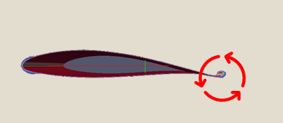
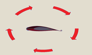
  The model resolves an important feature that the arrow points to in the figure below called a trailing (starter) vortex. It is this vortex that explains faster flow on the top surface of the wing. How it does this is described next.


  

  
  

  
  

  Here is what the computer model tells us

  
  

  
  

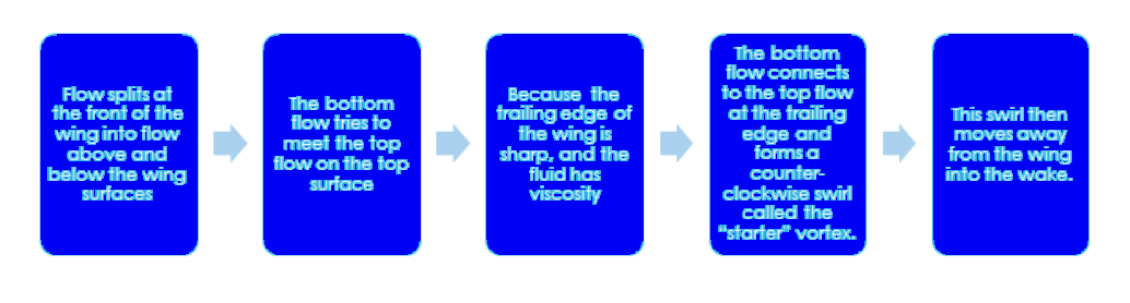
  Flow splits at the front of the wing into flow above and below the wing surfaces, the bottom flow tries to meet the top flow by flowing back around the sharp edge of the airfoil which would establish a second stagnation point on the top surface near the back edge. But due to real fluid properties, such as viscosity, it cannot flow back around the tailing edge even though it retains a counter-clockwise tendency. Instead, it connects to the top flow at the trailing edge forming a counter-clockwise swirl called the “starter” vortex which we see in the computer model. This vortex is predicted by aerodynamic theory as covered in the Clancy text. Once formed this vortex moves into the wake.

  
  

  
  

  
  

  The starting vortex that moves into the flow stream behind the wing is well known as wing tip vortices that present a hazard to closely following aircraft at airports.  In the 1970’s I was funded by NOAA to design an acoustic doppler transmitter, receiver warning device for installation on the main runway at Denver’s Stapleton airport. This device would detect the presence of the remains of the starter vortices by a reflected acoustical pulse.

  
  

  
  

  
  

  Wikipedia states “The origin of counter-rotating wing tip vortices is a direct and automatic consequence of the generation of lift by a wing”.

  
  

  A known consequence of the shedding vortex

  
  

  See the blurred image at the trailing edge of this planes wing - this is a visualization of the generation of lift.
  

  
  

• Lift is now explained

  

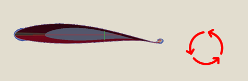
  When the starter vortex moves from the trailing edge, a clockwise vortex forms around the wing to conserve angular momentum. This clockwise vortex is called circulation.

  

  
  

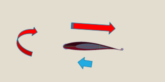
  The clockwise rotation of this circulation reinforces flow speed on the top of the wing and slows down flow on the bottom. Now we know why the top flow is faster!.

  
  

  
  

  Result - LIFT!
  

• Lift on Mars

  "What about lift on Mars?"
  

  Lift is directly proportional to density and velocity.  Since the density of the Martian atmosphere is much less than our own atmosphere (0.020 kg/m³ ), it would seem likely that lift on Mars would be much smaller, and that large blades swirling at high velocity would be needed.  Here is a picture of NASA's Martian helicopter and its specifications:
  

  

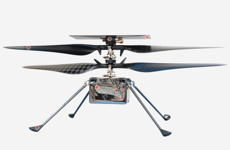
  Tech Specs

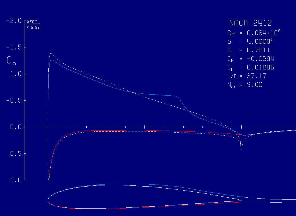
  Mass	1.8 kilograms
  Weight	4 pounds on Earth; 1.5 pounds on Mars
  Width	Total length of rotors: ~4 feet (~1.2 meters) tip to tip
  Power	Solar panel charges Lithium-ion batteries, providing enough energy for one 90-second flight per Martian day (~350 Watts of average power during flight)
  Blade span	Just under 4 feet (1.2 meters)
  Flight range	Up to 980 feet (300 meters)
  Flight altitude	Up to 15 feet (5 meters)
  Flight environment	Thin atmosphere, less than 1% as dense as Earth's

   

  
  

  
  

  
  

  
  

  
  

  The NASA Glenn Research Center has made available a JAVA program calculating lift on Mars as covered in the next section which confirms the loss of lift in the thin Martian atmosphere. Comparing lift for the same design airfoil, they found lift dropping to 1.2 % of the lift value for Earth.

  
  

  The MIT program for lift analysis called XFoil has been used to compare lift on Mars to lift on Earth by considering two Reynolds numbers (ρvL/μ) 500000 for Earth and 84000 for Mars (the correction for ρ/μ being .0168 with velocity  and the airfoil constant ). This program shows a L/D ratio of 37/121, or Martian lift is about 30% of lift on Earth corrected for density and viscosity. This higher result compared to the analysis from the Glenn program seems reasonable considering the successful flight of the helicopter on Mars.
  

  
  

  
  

  
  

  
  

  
  

  
  

• Models you can use

  The airfoil

  There are two airfoil sources on the internet:

  1. NACA airfoil generator

  2. UIUC Airfoil Data Site

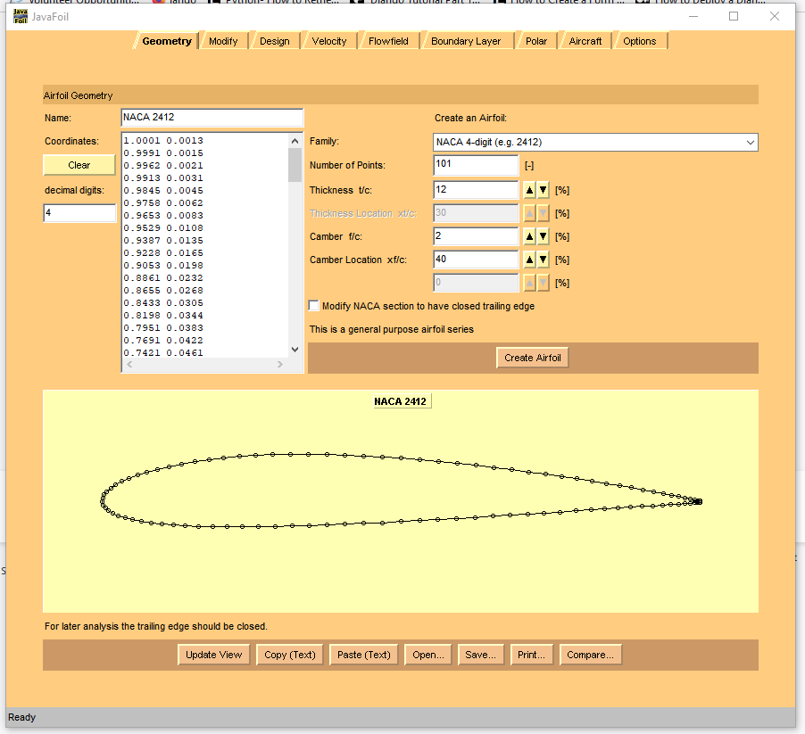
  I flew Blanic gliders, its airfoil is NACA 2412. This wing can be defined by source 1:

  
  

  Reynolds Number and other terms to know

  
  

  You should know the defining dimensions of a wing: wingspan (distance from wingtip to wingtip), chord (horizontal distance from leading to trailing edge which can be at the wing root, at the tip, or an average of these, a characteristic chord is computed from wingspan divided by chord which is called aspect ratio).

  
  

  To analyze airfoils by the three, free, programs that are available to you for downloading, you have to know the Reynolds number which characterizes flight speed. The Reynolds number for airfoils is:

  
  

  Re = V c / ν

  
  

  where V is the flight speed, c is the chord length, and ν is the kinematic viscosity of the fluid in which the airfoil operates, which is 1.460×10⁻⁵ m²/s for Earth's atmosphere at sea level.
  

  So, the Reynolds numbers to look for the Blanic wing include:  stall speed, 40 miles/hr, best lift speed ~70 miles/hr, and maximum flight speed, ~157miles/hr. The Reynolds number for these are:

  1,495,000
  2,660,000
  5,800,000
  

  
  

  
  

  FoilSim II from Glenn Research Center, NASA

  
  

  Lift simulation on Earth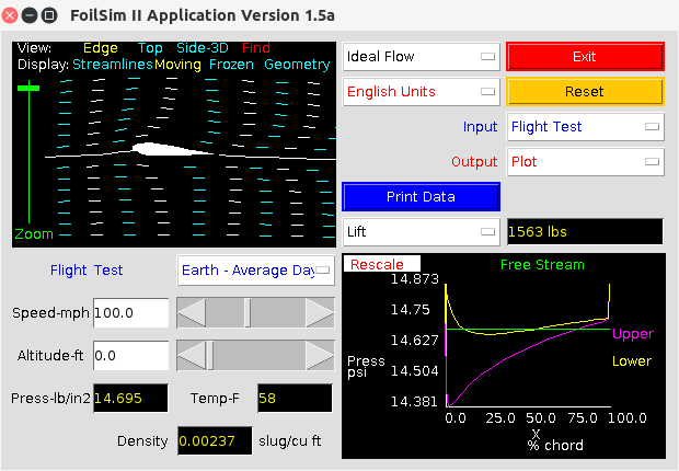

  
  

  
  

  
  

  Mars lift simulation

  
  

  

  This program will compute the change in lift for the average day atmospheres of Earth and Mars for a specific airfoil as shown in these views:

  Lift on Mars (left) vs. Lift on Earth (right)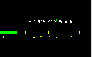

  
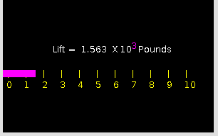
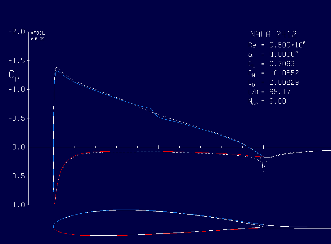
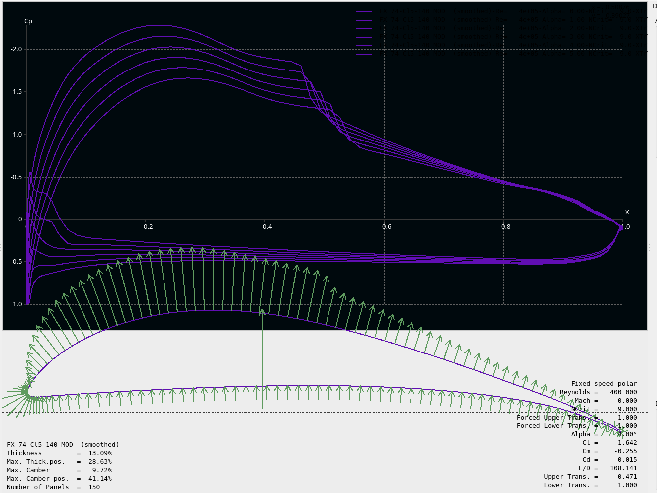
  This program expects the lift on Mars to be 19.3/1563.0 (pounds) or 1.23 % of that on Earth. This means a Martian helicopter needs wider blades that rotate much faster, and that its payload will be much smaller.
  

  Two other programs may interest you: MIT has developed XFoil (scripted, and just for analysis of a wing), and XFLR5 (with a Graphic Interface, GUI; for analysis of both a wing and a plane having three airfoils, wing, elevator and fin). Unfortunately, XFLR5 is much harder to learn. Below is a screencopy of a wing from the analysis in XFoil showing the distribution of pressure on the wing surfaces.
  

  XFLR5 from MIT
  

  

  
  

  JAVAFOIL
  

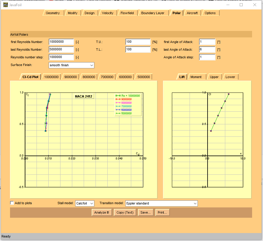
  The third program of interest is a java program called JAVAFOIL. It does an extensive wing analysis similar to XFLR5, but not a complete plane. It is much easier to learn to use. Following are screencopies

  
  

  
  

  Student project ideas

  
  

  You might get interested in the physics of flying, and flying yourself. Consider visiting your local soaring club if you live near one. Most clubs are happy to provide demonstration flights in two person training gliders with seasoned instructors for less than $50.00 (as my club in Houston did). You can prepare for this by reading soaring books like "The Joy of Soaring" (which is a training manual, but is in most large public libraries), or "Once Upon a Thermal" the story of a nearly 50 years old man, Richard Wolters, who took up soaring and became famous.

  
  

  On a demo flight you will experience stalls, and maybe spins (if you want), but surely you will experience thermalling which is gaining altitude by circling slowly and tightly with flaps out over terrain that produces a rising hot air column like a freshly plowed field, or a superstore black asphalt parking lot. Gliders have a special instrument called a variometer that displays vertical climb, and beeps when the glider passes over these columns of rising air - that's how gliders stay up and can cross hundreds of miles in daylight.

  
  

  Then you can analyze the performance of the glider's wing with one, or more, of the programs above. If you're really adventurous you can go further to use xflr5 (the big brother of xfoil) to analyze the complete wing, or even the complete plane. Below is an example of an analysis by xflr5 of a complete wing: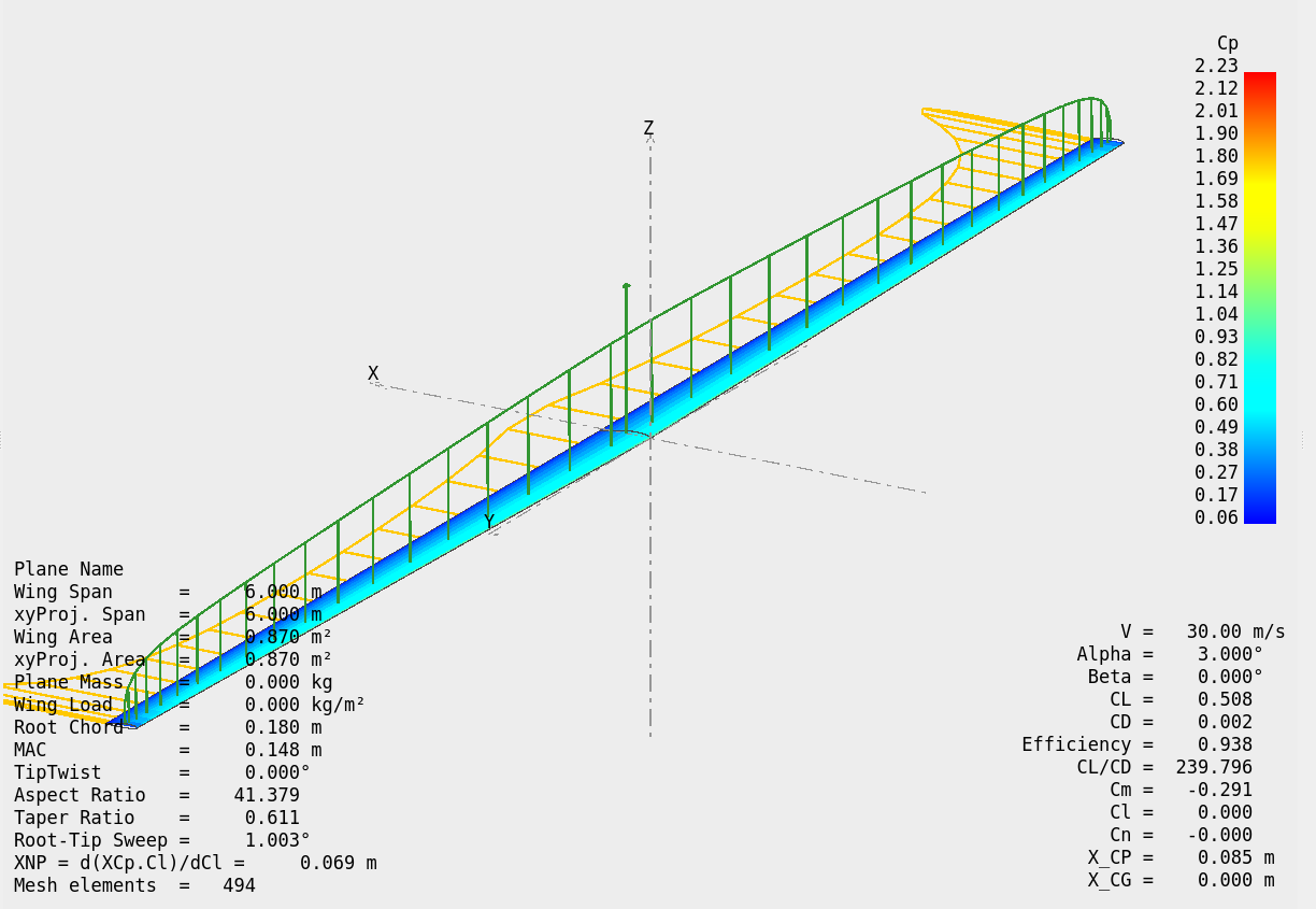

  
  

  
  

  
  

  You can make a large poster of your project for display at your school's science fair, (the American Society of Mechanical Engineers, ASME, even has opportunities for poster displays in ASME conferences that include junior contrbutions). Have you wondered how these large colorful posters are made? This is how: in Powerpoint made a large slide, add your graphics and text to it, then print the slide with a large format HP printer. (such as HP Designjet 630)
  

  
  

  
  

• References

  There exists many texts and papers supporting this lecture, but two stand out. The first is Clancy’s classic textbook on this subject intended for British aeronautics students. You will find a very detailed development of flow around cylinders, spheres and airfoils. The second reference follows this one as a validation of the ideas presented here. Also referenced are internet sources for the free airfoil programs.
  

  1. https://www.grc.nasa.gov/www/k-12/airplane/foil3.html (FoilSim from Glenn Research Center)
  2. https://web.mit.edu/drela/Public/web/xfoil/ (XFoil from MIT)
  3. https://www.mh-aerotools.de/airfoils/javafoil.htm (JAVAFOIL)
  4. Aerodynamics, L.J. Clancy, John Wiley & Sons, New York, 1975
  5. MIT presentation - Reports on how things work - by Mealani Nakamura entitled "Air Foil"
     

  
  

  
  

• Quiz
  Página: 1

• Send a Postcard to Space!

  Send a Postcard to Space through NSS Supported Blue Origin Club For The Future initiative!

  Visit: SpacEdge Academy Postcards in Space Course