Educator Onboarding
LEO Art Challenge Workshop
Satellite Tracking, Orbits, and Modeling
Workshop: Satellite Tracking, Orbits, and Modeling
Workshop: Trek-a-Sat
Workshop: Yerkes
Workshop: Electrostatics in Space - Carthage- Yerkes
Workshop: Life in Space! BTCI
Workshop: More Than a Rainbow - Yerkes
Workshop: Small Steps Teachimg Space Brings Giant Steps in Classrooms-SEEC
Workshop: 2017-01-28 Yerkes
Tools You Might Use
Educational Learning
Standards
Documentation
Newton's Greatest Contribution to Humankind
विषयवस्तु
-
Isaac Newton proves that Kepler's orbit of Mars is heliocentric and ushers in the Age of Reason.
-
Author - Peter Higgins, PhD
Isaac Newton contributed much to science, and is revered for many contributions in mechanics, Newton's 3 laws, optics,
invention of a reflecting telescope, physics, nature of light, mathematics, extension of the binomial theorem
and a form of calculus, and heat transfer, Newton's Law of Cooling. By far, though, Newtons greatest contribution was to prove Kepler and Copernicus were right thereby establishing that planets orbit the sun. The Ptolemaic model was vanquished, and ushered in the Age of Reason.
This lesson is the story of how this happened, and specifically, how Newton proved the orbit of Mars is elliptical with the Sun at a focal point. At the end of this lesson you will be able to produce his proof using Excel and a simple Python program.
Prerequisite: The lesson targets students who have been introduced to calculus and have some knowledge of astronomy. Both teachers and students should know Excel cell and simple Python coding. The excel book, and the python code are available as downloads from lesson files. In this lesson elementary numerical analysis by step wise iteration is introduced as a method for predicting the orbit. This is how orbital mechanics calculations are done. Some will be satisfied by the story itself, and some can learn the scientific method of problem solving that involves clearly stating the objectives, drawing a force diagram, stating the relevant equations then applying them. Hopefully, students will be challenged to learn more - maybe even to become cosmologists!Age Level for the lesson: 14+
Next Generation Science Standards:
HS-ESS1-4 - Use mathematical or computational representations to predict the motion of orbiting objects in the solar system.
Keywords:
Newton, Wren, Kepler, Copernicus, Mars, scientific method, orbital mechanics, force diagram, Python
For further study: Interactive site for educators and students:
http://microcosmos.uchicago.edu/microcosmos_new/index.html
-
About Newton
Newton was born in the United Kingdom, and lived from 1642 (the year Galileo died) until 1727. He was considered both the first of the Age of Reason joining the likes of Laplace, and the last of the alchemists-astrologers who bedazzled Europe’s royalty. He was a lonely figure, and a mystic. People of that time still tried to avoid the plague and Newton certainly did. He was envied by many, especially Robert Hooke, who tried to claim credit for much of what Newton did such as the monumental proof presented here.
Newton’s contributions
Isaac Newton was remarkable for fundamental contributions in mathematics and statistics, optics, mechanics, cosmology, and thermodynamics. In much of these contributions his work was a continuation of the work of others before him, but because at that time attribution of the work of others wasn’t common, it is sometimes unclear what Newton added to a field that came uniquely from him.
Some examples:
• Binomial expansions had been known dating back to Euclid in the 4th century B.C. Newton’s contribution was to generalize the exponent to any rational number.
• Newton invented a reflecting telescope design in 1666, but John Gregory conceived an alternative reflector design before Newton in 1663.
• Newton was first to understand that the rainbow of colors from a prism was not made by the prism but were spectral components of light. Others before him had seen the rainbow of colors from a prism, but didn’t understand them. Unfortunately, Newton was so convinced that light consisted only of particles that the wave nature of light was not considered for some time. This is interesting because it is the wave nature of light which accounts for its separation into colors by refraction in the prism.
• Newton’s three laws of mechanics included the ideas of Galileo, especially on inertia.
• Liebniz is believed to have coinvented calculus publishing his formulations in 1684 which preceded publication of Newton’s papers on calculus by 27 years. Further it is Liebniz’s symbolic form of calculus, such as those for integration and differentiation that are used today.
• In the journal Heat Transfer Engineering it is mentioned that “Boyle gave a qualitative demonstration of the principle known as Newton’s law of cooling in his book, Experiments Touching Cold in 1665” which preceded Newton’s publication of the cooling law in 1701.
Newton’s greatest contribution to humankind
In contrast to what is accepted now as truth from valid experimental results or observations, science in Newton’s day discounted these in favor of theory. So Kepler’s reduction of Tycho Brahe’s observations of the daily celestial position of Mars, which established its trajectory to be an ellipse having the sun as a focal point, was not considered then as a fact. Instead Kepler’s findings were taken as only describing the data, i.e. an explanation of the data. In the same way, Copernicus's conclusion upon updating the Ptolemaic tables that a heliocentric planetary model made sense was discounted as mere convenience. The church insisted that planetary motion, based on the perfection of circular orbits, was irrefutable unless such motion as suggested by Kepler could be proven using secular logic beyond any doubt. Up to Newton’s time a proof fitting this criteria was unknown for at least two reasons and one logical criticism. The two reasons were (1) the mathematics of objects in motion didn’t exist, and (2) gravitational force was not qualified. Of course, the pull of gravity was known, and Galileo was exploring it, but its role in determining a planet’s motion was not. The universally held criticism was the incongruity that the Earth could be hurtling through space at over 14 thousand m/s. At such a speed, it was reasoned, why wasn’t everything blown away?
Others in this story
Hipparchus
 Hipparchus, Greek astronomer, around 100 B.C. duplicated his observations of planetary motion by proposing the idea that the planets were each frozen in a separate sphere which was contained in another separate larger sphere that revolved about a point near Earth. Matching his model to observation was accomplished by adjusting the speeds of rotation of the two spheres. He named the small sphere the epicycle and the large sphere the deferent.
 Tycho Brahe
Tycho Brahe called the best naked-eye astronomer made meticulous observations of planetary position in the late 16th century. He was a quarrelsome Danish nobleman who lost his nose in a dual over mathematics when he was nineteen. At the end of his life he passed on his observations to Kepler for making tables of planetary motion.Johann Kepler
Johann Kepler, a German (1571-1630) mystic astrologer and astronomer, brilliant in mathematics and whose mother was tried as a witch, published Tycho's tables of planetary motion in 1609 in which he claimed Mars to follow an elliptical orbit having the Sun at a focal point.
Nicolas Copernicus
Nicholas Copernicus is famous for beginning the Scientific Revolution. As early as 1507, while working to revise the Ptolemaic tables of planetary motion, he concluded that a heliocentric model of the universe would explain the retrograde motion of Mars much easier than laborious contortions of epicycles and deferents. Eventually his theories were published, but the truth of them was not accepted by the church. See the excellent book on this story entitled "The Book Nobody Read", by the scientist-historian Owen Gingerich. -

From Greek until Newton’s time, the accepted view of planetary motion followed the Ptolemaic system. Originally proposed around 140 B.C. by Hipparchus (the greatest of the Greek astronomers) each planet orbited Earth bound by a circle, the epicycle, which in turn, was included in a larger circle, the deferent. Tables describing the position of each planet on these circles, along with methods for combining them, were formalized by Claudius Ptolemy some hundred years later and Hipparchus’ system now bears his name. These tables had to be corrected periodically to maintain accuracy, and it was in doing so that Copernicus proposed a much simpler alternative – a heliocentric system. The Ptolemaic system was especially important because astrology depended upon it, and the royal courts depended on astrology1. Most astronomers of that time were astrologers. The Ptolemaic system is complicated but it is so accurate that it is still used by planetariums. Its accuracy is another reason for not abandoning it.
1Astrology is a method of predicting mundane events based upon the assumption that the celestial bodies—particularly the planets and the stars considered in their arbitrary combinations or configurations (called constellations)—in some way either determine or indicate changes in the sublunar world.
-
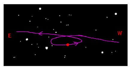
A curious thing happens when an observer records the position of Mars each night: About every 26 months, Mars appears to make a loop in the sky. Hipparchus accounted for this motion using an epicycle within the deferent. But, the loop is only the consequence of the relative positions of Earth and Mars in their orbits when Earth passes by Mars. Earth is orbiting the Sun about twice as fast as Mars orbits the Sun. About every 26 months, Earth comes up from behind and overtakes Mars. Normally, Mars appears to move from East to West, but in this 26 month overtaking Mars appears to move from West to East as Earth overtakes Mars
By projection this anomaly is apparent as a consequence of the orbital speeds when considering a heliocentric point of view.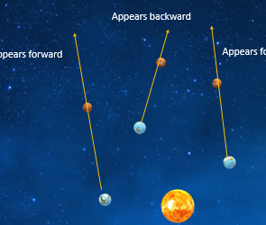
-
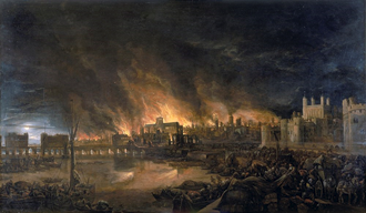
Shorty after 1666, Christopher Wren, made wealthy and famous as the architect of London following the great London fire offered a prize to anyone proving that conventional forces (not angels) were responsible for planetary motion explained by Johann Kepler in 1609. To be accepted the proof had to use secular ideas and mathematics (no magic, no divine intervention). Both Hooke and Newton claimed a proof, but only Newton produced it.
-
The force diagram
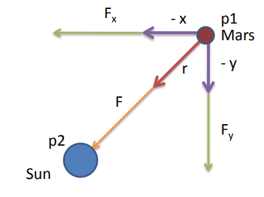
A force is required to alter the course of a body according to laws of inertia. A force diagram aids in understanding how Mars changes direction to follow a path in space. All objects near Mars exert a gravitational force on it including the Sun, Earth and Jupiter, but of these, the pull of the Sun dominates exerting well over 99 % of the gravitational force on Mars. Newton stated that the gravitational force between objects is proportional to the product of their masses divided by the square of the distance between them. The Greek mathematician Thales of Miletus was first to recognize similar triangles – using this identity we can relate the force components to the distance components, equation 2, because their angles are the same. Mars, mass equal m, is at point p1, a distance r from the Sun having mass equal M, at point p2. F is the force of gravity given by newton as:
F=GMm/r2 (1)
Fx and Fy are the x,y components of F. –x and –y are the components of r since F and r are vectors. According to similarity:
Fx / F = - x / r and Fy / F = - y / rmultiplying by F we get:Fx = - Fx / r and Fy = -F y / r (2)Formulas for the components of acceleration needed in the proof
From Newton’ 2nd law, we get F = m a (3)
therefore dividing both sides by mass, a = F / m, and in component form, ax = Fx / m, ay = Fy / m
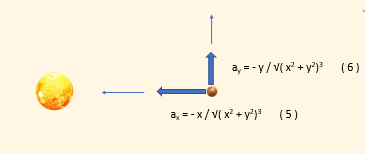
Substituting the components of (1) into the components of (2), and considering the approximation GM == 1, we arrive at: - an exercise for students
ax = -x / r3 (4)
and
ay = -y / r3 (5)
To apply them to get increments of position change using Newton’s calculus
ax = Δvx / Δt and ay = Δvy / Δt
rearranging to:
Δvx = axΔt and Δvy = ayΔt (6)
which computes computes velocity increments. To get velocity at the new point we add the velocity increment to the last velocity:
for x
vx,p = vx,p-1 + Δvx (7)
for y
vy,p = vy,p-1 + Δvy (8)
by the same method to get the new position increment
Δpx = vx Δt and Δpy = vy Δt (9)
and the new position by adding increment to last positionfor x
xx,p = x,p-1 + Δpx (10)
for y
yy,p = yy,p-1 + Δpy (11)
Setting up the proof
The problem is set up by redrawing the force diagram for the starting position, and by using the force equations found earlier. It is reasoned that its subsequent displacement will be uniquely determined by only the forces acting on it. This is concluded from studies by Galileo and summarized in Newton’s 2nd law which states that a force is required to change the speed or direction of a body at rest or in motion. It is somewhat curious that Newton used only gravitational forces to determine displacement and did not include a drag term even though he introduced the substance Luminiferous aether to support light propagation in space. Perhaps it was realized that if a drag force existed then the planetary orbits would degrade which observations don’t support. In defense of the religious notion that angels guided the planets in circular paths, it would follow that they could overcome drag effects by pushing harder.
Initial conditions
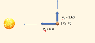
Remember this proof is only required to show that secular laws can correctly predict movement of the planet. Since the proof is not required to match the observed celestial positions relative to the Sun, the values for initial conditions are arbitrary.
Three steps needed in the solution
o Compute a from x, y position at dt
o Compute new v = old v + a dt
o Compute new position = old position + v dt
-
Calculations using Excel
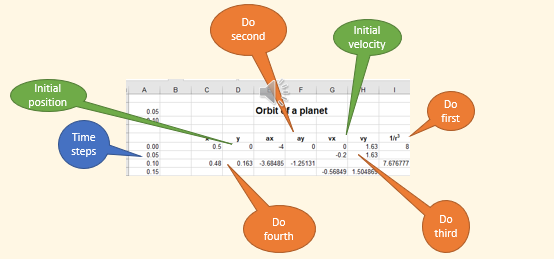
Excel can be used for these calculations. Functions performed on the spreadsheet are identified by markers. First 1/r3 is calculated with r replaced with √(x2 + y2). Second, acceleration components are computed by multiplying 1/r3 by -x and –y (equations 5 and 6). Third, the new velocity is found by adding Δv which is acceleration times the timestep, Δt (0.05 for first step, 0.1 all other steps) to the last velocity. The last calculation for this time is to determine the new position by adding Δp (= v times Δt) to the last p. Programming these calculations is done by inserting instructions in cells as shown next.
Programming Excel Sheet
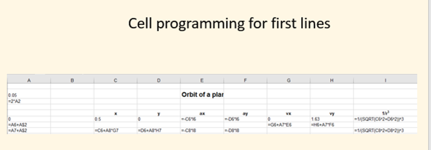
Type these instructions into the cells indicated; for example, type “=C6+A8*G7” into cell C8 for the new x position.
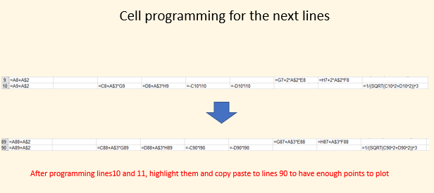
Now program rows 9 and 10 exactly as shown here. When done, highlight these two rows (9 and 10) and paste them into rows 11-90.
Plot the results
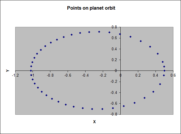
To finish, to the right of the columns just constructed, program the spreadsheet to plot the x and y columns by identifying them as plot ranges. Set the spreadsheet to calculate automatically and the plot of x, y points that compose the orbit will appear.
Calculating with Python
A simple python program that does the same calculations as the Excel sheet described above.First the python packages needed by computations are imported. Sometimes these imports will fail to find these packages; in which case, they must be included by either using the package manager of the IDE, or by “pip install package-name” from the terminal. Next the arrays (lists) needed to store results such as positions are declared. These declarations are mandatory. Lastly, the initial conditions are entered.
Running the python program produces the plot below:A simple python program import re
import matplotlib.pyplot as plt
import numpy as np
import PyGnuplot as gp
import mathimport needed modules
Px=[]
Py=[]
Pvx=[]
Pvy=[]
R=[]
A=[]
Ax=[]
Ay=[]
Vx=[]
Vy=[]initialize the arrays used to store results
x=(float(0.5))
y=(float(0.0))
vx=(float(0.0))
vy=(float(1.63))initial conditions #1st iteration, half step in time
ax=(-float(x/(math.sqrt(x**2 + y**2))**3))
ay=(-float(y/(math.sqrt(x**2 + y**2))**3))
dt0=0.05
Vx=(ax*dt0)+vx
Vy=(ay*dt0)+vy
dt1=0.1
X=x+(Vx*dt1)
Y=y+(Vy*dt1)
Px.append(x)
Px.append(X)
Py.append(y)
Py.append(Y)
Pvx.append(Vx)
Pvy.append(Vy)
Pvx.append(Vx)
Pvy.append(Vy)
print(x, y, X, Y)for i in range(1,90):
ax=(-float(Px[i]/(math.sqrt(Px[i]**2 + Py[i]**2))**3))
ay=(-float(Py[i]/(math.sqrt(Px[i]**2 + Py[i]**2))**3))
Pvx.append(ax*dt1+Pvx[i-1])
Pvy.append(ay*dt1+Pvy[i-1])
Px.append(Px[i-1]+(Pvx[i]*dt1))
Py.append(Py[i-1]+(Pvy[i]*dt1))
plt.plot(Px,Py,'*b')
ax=plt.gca()
ax.set_facecolor('lightgray')
ax.axhline(y=0, color='g')
ax.axvline(x=0, color='g')
plt.title("Orbit plot of x, y points")
plt.grid()
plt.show()Now, the problem calculations are defined to process initial conditions, and the results appended to lists. The print statement is a diagnostic and can be commented out with a #.A for loop extends the calculations for an entire orbit. The loop is terminated by a : followed by indentation of statements comprising the loop. Lastly the lists are plotted.
-
- Another look at this:https://spacedge.nss.org/course/view.php?id=50
- A working Excel sheet: orbit.xls
- The python program: newtonMarsOrbit.py
- ‘the Feynman Lectures on Pysics’, Addison Wesley, 9-6
- Asimov’s Biographical Encyclopedia Of Science & Techology, Doubleday
- An on-line Python tutorial: https://docs.python.org/3/tutorial/
-
Send a Postcard to Space through NSS Supported Blue Origin Club For The Future initiative!
Visit: SpacEdge Academy Postcards in Space Course